本文旨在通過最通俗易懂的過程來詳解Transformer的每個步驟！

假設我們在做一個從中文翻譯到英文的過程，我們的詞表很簡單如下：

中文詞表：[機、器、學、習] 英文詞表[deep、machine、learning、chinese]

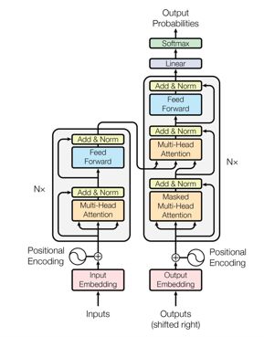
先來看一下Transformer的整個過程：

接下來，我們將按順序來講解Transformer的過程，并配有配套的excel計算過程和tensorflow代碼。

先說明一下，本文的tensorflow代碼中使用兩條訓練數據（因為實際場景中輸入都是batch的），但excel計算只以第一條數據的處理過程為例。

1、Encoder輸入

Encoder輸入過程如下圖所示：

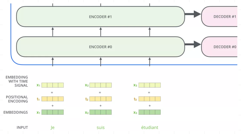
首先輸入數據會轉換為對應的embedding，然后會加上位置偏置，得到最終的輸入。

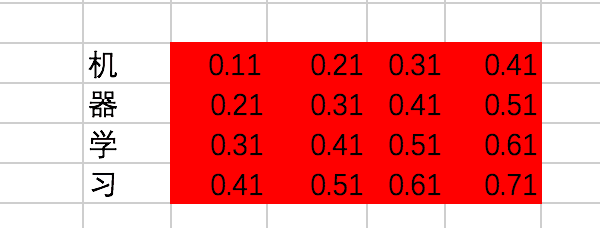
這里，為了結果的準確計算，我們使用常量來代表embedding，假設中文詞表對應的embedding值分別是：

位置偏置position embedding使用下面的式子計算得出，注意這里位置偏置是包含兩個維度的，不僅僅是encoder的第幾個輸入，同時embedding中的每一個維度都會加入位置偏置信息：

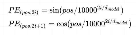
不過為了計算方便，我們仍然使用固定值代替：

假設我們有兩條訓練數據（Excel大都只以第一條數據為例）：

[機、器、學、習] -> [ machine、learning][學、習、機、器] -> [learning、machine]

encoder的輸入在轉換成id后變為[[0,1,2,3],[2,3,0,1]]。

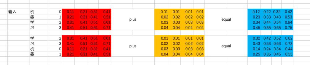
接下來，通過查找中文的embedding表，轉換為embedding為：

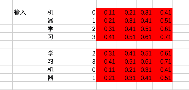
對輸入加入位置偏置，注意這里是兩個向量的對位相加：

上面的過程是這樣的，接下來咱們用代碼來表示一下：

import tensorflow as tfchinese_embedding = tf.constant([[0.11,0.21,0.31,0.41], [0.21,0.31,0.41,0.51], [0.31,0.41,0.51,0.61], [0.41,0.51,0.61,0.71]],dtype=tf.float32)english_embedding = tf.constant([[0.51,0.61,0.71,0.81], [0.52,0.62,0.72,0.82], [0.53,0.63,0.73,0.83], [0.54,0.64,0.74,0.84]],dtype=tf.float32)position_encoding = tf.constant([[0.01,0.01,0.01,0.01], [0.02,0.02,0.02,0.02], [0.03,0.03,0.03,0.03], [0.04,0.04,0.04,0.04]],dtype=tf.float32)encoder_input = tf.constant([[0,1,2,3],[2,3,0,1]],dtype=tf.int32)with tf.variable_scope("encoder_input"): encoder_embedding_input = tf.nn.embedding_lookup(chinese_embedding,encoder_input) encoder_embedding_input = encoder_embedding_input + position_encodingwith tf.Session() as sess: sess.run(tf.global_variables_initializer()) print(sess.run([encoder_embedding_input]))

結果為：

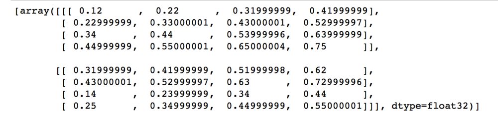
跟剛才的結果保持一致。

2、Encoder Block

一個Encoder的Block過程如下：

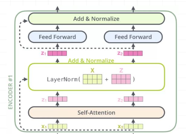
分為4步，分別是multi-head self attention、Add & Normalize、Feed Forward Network、Add & Normalize。

咱們主要來講multi-head self attention。在講multi-head self attention的時候，先講講Scaled Dot-Product Attention，我有時候也稱為single-head self attention。

2.1 Attention機制簡單回顧

Attention其實就是計算一種相關程度，看下面的例子：

Attention通常可以進行如下描述，表示為將query(Q)和key-value pairs映射到輸出上，其中query、每個key、每個value都是向量，輸出是V中所有values的加權，其中權重是由Query和每個key計算出來的，計算方法分為三步：

1）計算比較Q和K的相似度，用f來表示：

2）將得到的相似度進行softmax歸一化：

3）針對計算出來的權重，對所有的values進行加權求和，得到Attention向量：

計算相似度的方法有以下4種：

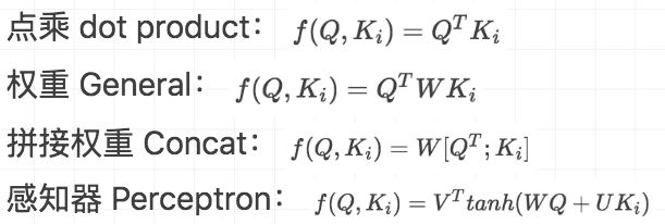
在本文中，我們計算相似度的方式是第一種。

2.2 Scaled Dot-Product Attention

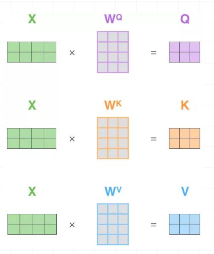
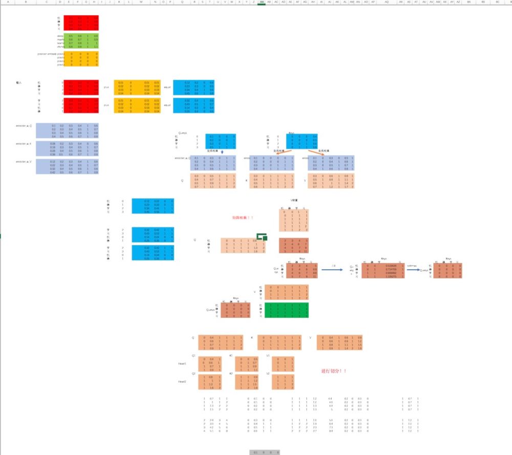
咱們先說說Q、K、V。比如我們想要計算上圖中machine和機、器、學、習四個字的attention，并加權得到一個輸出，那么Query由machine對應的embedding計算得到，K和V分別由機、器、學、習四個字對應的embedding得到。

在encoder的self-attention中，由于是計算自身和自身的相似度，所以Q、K、V都是由輸入的embedding得到的，不過我們還是加以區分。

這里， Q、K、V分別通過一層全連接神經網絡得到，同樣，我們把對應的參數矩陣都寫作常量。

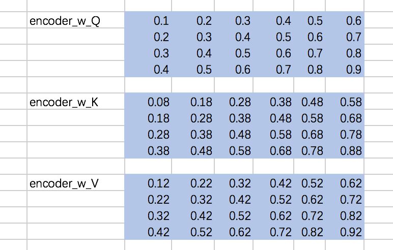
接下來，我們得到的到Q、K、V，我們以第一條輸入為例：

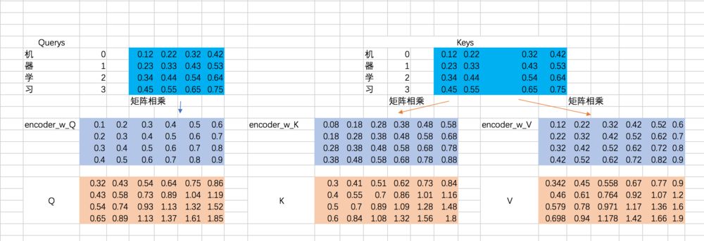
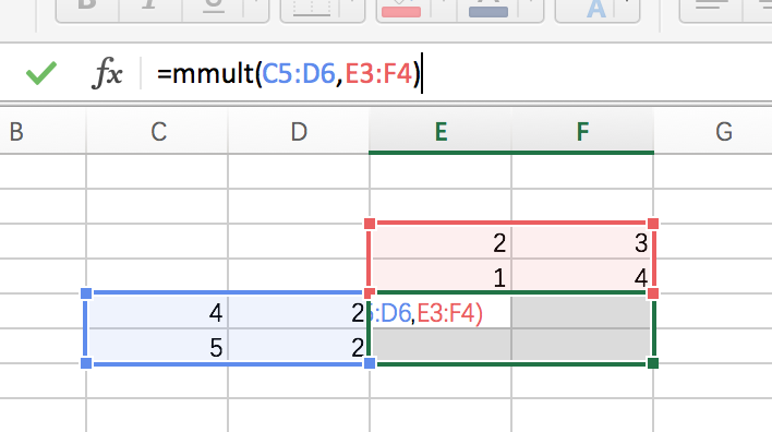
既然是一層全連接嘛，所以相當于一次矩陣相乘，excel里面的矩陣相乘如下：

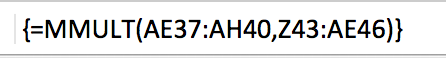
在Mac中，一定要先選中對應大小的區域，輸入公式，然后使用command + shift + enter才能一次性得到全部的輸出，如下圖：

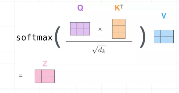
接下來，我們要去計算Q和K的相關性大小了，這里使用內積的方式，相當于QKT:

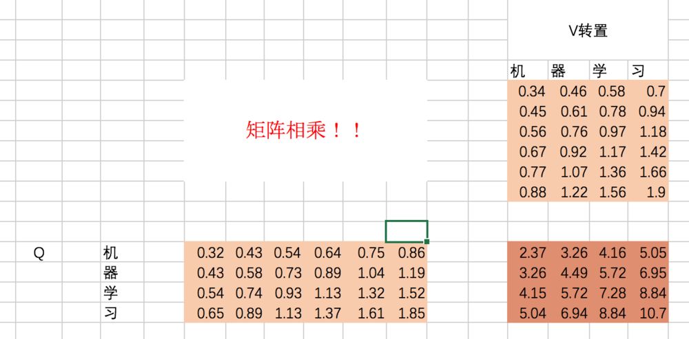
(上圖應該是K,不影響整個過程理解)同樣，excel中的轉置，也要選擇相應的區域后，使用transpose函數，然后按住command + shift + enter一次性得到全部輸出。

我們來看看結果代表什么含義：

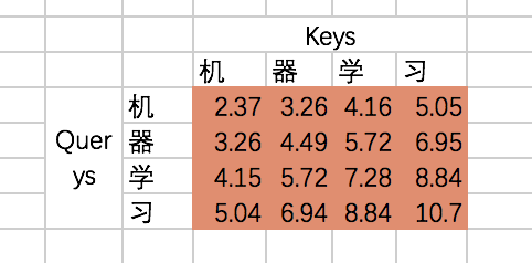
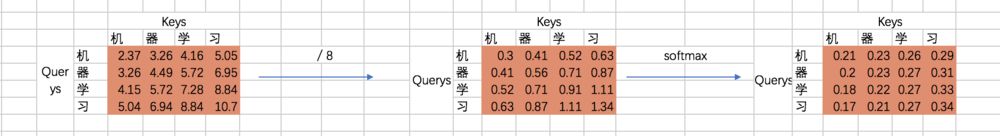
也就是說，機和機自身的相關性是2.37(未進行歸一化處理),機和器的相關性是3.26，依次類推。我們可以稱上述的結果為raw attention map。對于raw attention map，我們需要進行兩步處理，首先是除以一個規范化因子，然后進行softmax操作，這里的規范化因子選擇除以8，然后每行進行一個softmax歸一化操作（按行做歸一化是因為attention的初衷是計算每個Query和所有的Keys之間的相關性)：

最后就是得到每個輸入embedding 對應的輸出embedding，也就是基于attention map對V進行加權求和，以“機”這個輸入為例，最后的輸出應該是V對應的四個向量的加權求和：

如果用矩陣表示，那么最終的結果是規范化后的attention map和V矩陣相乘，因此最終結果是：

至此，我們的Scaled Dot-Product Attention的過程就全部計算完了，來看看代碼吧：

with tf.variable_scope("encoder_scaled_dot_product_attention"): encoder_Q = tf.matmul(tf.reshape(encoder_embedding_input,(-1,tf.shape(encoder_embedding_input)[2])),w_Q) encoder_K = tf.matmul(tf.reshape(encoder_embedding_input,(-1,tf.shape(encoder_embedding_input)[2])),w_K) encoder_V = tf.matmul(tf.reshape(encoder_embedding_input,(-1,tf.shape(encoder_embedding_input)[2])),w_V) encoder_Q = tf.reshape(encoder_Q,(tf.shape(encoder_embedding_input)[0],tf.shape(encoder_embedding_input)[1],-1)) encoder_K = tf.reshape(encoder_K,(tf.shape(encoder_embedding_input)[0],tf.shape(encoder_embedding_input)[1],-1)) encoder_V = tf.reshape(encoder_V,(tf.shape(encoder_embedding_input)[0],tf.shape(encoder_embedding_input)[1],-1)) attention_map = tf.matmul(encoder_Q,tf.transpose(encoder_K,[0,2,1])) attention_map = attention_map / 8 attention_map = tf.nn.softmax(attention_map)with tf.Session() as sess: sess.run(tf.global_variables_initializer()) print(sess.run(attention_map)) print(sess.run(encoder_first_sa_output))

第一條數據的attention map為：

第一條數據的輸出為：

可以看到，跟我們通過excel計算得到的輸出也是保持一致的。

咱們再通過圖片來回顧下Scaled Dot-Product Attention的過程：

2.3 multi-head self attention

Multi-Head Attention就是把Scaled Dot-Product Attention的過程做H次，然后把輸出Z合起來。

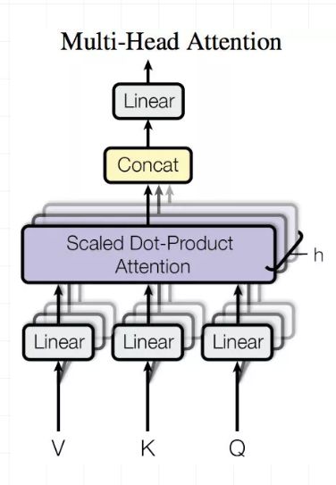
整個過程圖示如下：

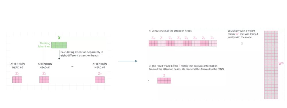
這里，我們還是先用excel的過程計算一遍。假設我們剛才計算得到的Q、K、V從中間切分，分別作為兩個Head的輸入：

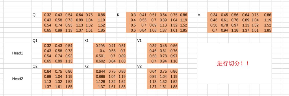
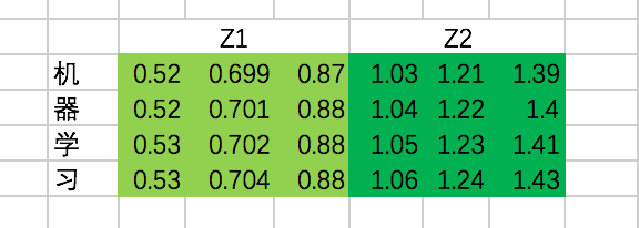
重復上面的Scaled Dot-Product Attention過程，我們分別得到兩個Head的輸出：

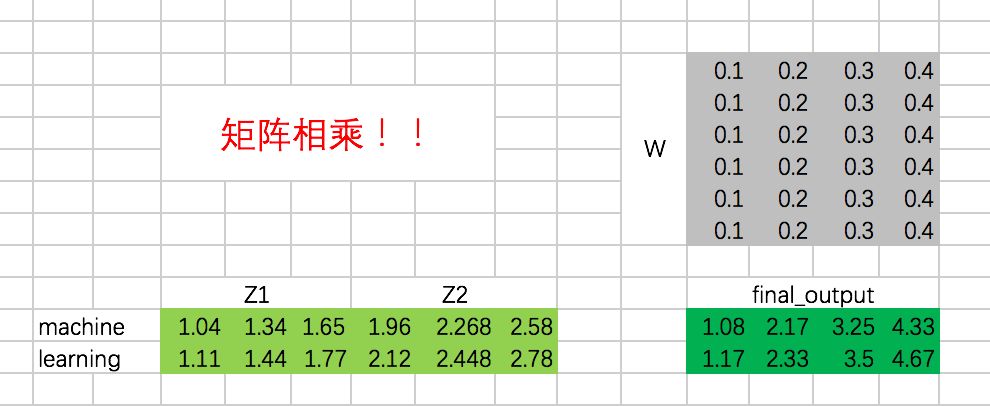
接下來，我們需要通過一個權重矩陣，來得到最終輸出。

為了我們能夠進行后面的Add的操作，我們需要把輸出的長度和輸入保持一致，即每個單詞得到的輸出embedding長度保持為4。

同樣，我們這里把轉換矩陣W設置為常數：

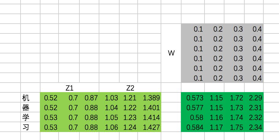
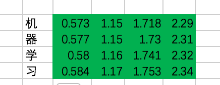
最終，每個單詞在經過multi-head attention之后，得到的輸出為：

好了，開始寫代碼吧：

w_Z = tf.constant([[0.1,0.2,0.3,0.4], [0.1,0.2,0.3,0.4], [0.1,0.2,0.3,0.4], [0.1,0.2,0.3,0.4], [0.1,0.2,0.3,0.4], [0.1,0.2,0.3,0.4]],dtype=tf.float32)with tf.variable_scope("encoder_input"): encoder_embedding_input = tf.nn.embedding_lookup(chinese_embedding,encoder_input) encoder_embedding_input = encoder_embedding_input + position_encodingwith tf.variable_scope("encoder_multi_head_product_attention"): encoder_Q = tf.matmul(tf.reshape(encoder_embedding_input,(-1,tf.shape(encoder_embedding_input)[2])),w_Q) encoder_K = tf.matmul(tf.reshape(encoder_embedding_input,(-1,tf.shape(encoder_embedding_input)[2])),w_K) encoder_V = tf.matmul(tf.reshape(encoder_embedding_input,(-1,tf.shape(encoder_embedding_input)[2])),w_V) encoder_Q = tf.reshape(encoder_Q,(tf.shape(encoder_embedding_input)[0],tf.shape(encoder_embedding_input)[1],-1)) encoder_K = tf.reshape(encoder_K,(tf.shape(encoder_embedding_input)[0],tf.shape(encoder_embedding_input)[1],-1)) encoder_V = tf.reshape(encoder_V,(tf.shape(encoder_embedding_input)[0],tf.shape(encoder_embedding_input)[1],-1)) encoder_Q_split = tf.split(encoder_Q,2,axis=2) encoder_K_split = tf.split(encoder_K,2,axis=2) encoder_V_split = tf.split(encoder_V,2,axis=2) encoder_Q_concat = tf.concat(encoder_Q_split,axis=0) encoder_K_concat = tf.concat(encoder_K_split,axis=0) encoder_V_concat = tf.concat(encoder_V_split,axis=0) attention_map = tf.matmul(encoder_Q_concat,tf.transpose(encoder_K_concat,[0,2,1])) attention_map = attention_map / 8 attention_map = tf.nn.softmax(attention_map) weightedSumV = tf.matmul(attention_map,encoder_V_concat) outputs_z = tf.concat(tf.split(weightedSumV,2,axis=0),axis=2) outputs = tf.matmul(tf.reshape(outputs_z,(-1,tf.shape(outputs_z)[2])),w_Z) outputs = tf.reshape(outputs,(tf.shape(encoder_embedding_input)[0],tf.shape(encoder_embedding_input)[1],-1)) import numpy as npwith tf.Session() as sess:# print(sess.run(encoder_Q))# print(sess.run(encoder_Q_split)) #print(sess.run(weightedSumV)) #print(sess.run(outputs_z)) print(sess.run(outputs))

結果的輸出為：

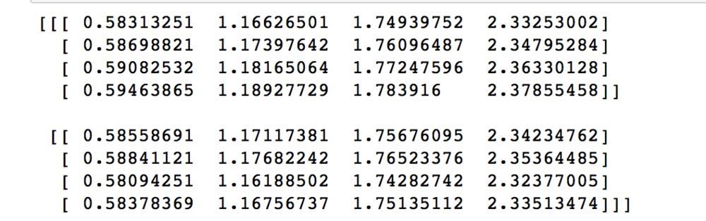
這里的結果其實和excel是一致的，細小的差異源于excel在復制粘貼過程中，小數點的精度有所損失。

這里我們主要來看下兩個函數，分別是split和concat，理解這兩個函數的過程對明白上述代碼至關重要。

split函數主要有三個參數，第一個是要split的tensor，第二個是分割成幾個tensor，第三個是在哪一維進行切分。也就是說， encoder_Q_split = tf.split(encoder_Q,2,axis=2)，執行這段代碼的話，encoder_Q這個tensor會按照axis=2切分成兩個同樣大的tensor，這兩個tensor的axis=0和axis=1維度的長度是不變的，但axis=2的長度變為了一半，我們在后面通過圖示的方式來解釋。

從代碼可以看到，共有兩次split和concat的過程，第一次是將Q、K、V切分為不同的Head：

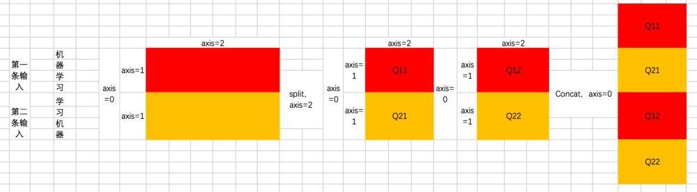
也就是說，原先每條數據的所對應的各Head的Q并非相連的，而是交替出現的，即 [Head1-Q11,Head1-Q21,Head2-Q12,Head2-Q22]

第二次是最后計算完每個Head的輸出Z之后，通過split和concat進行還原，過程如下：

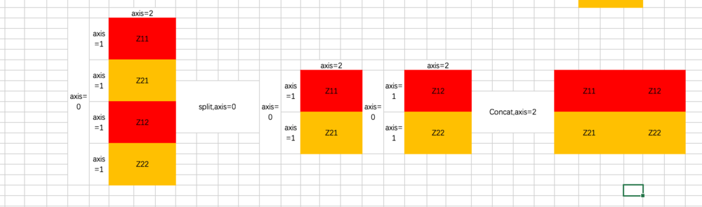
上面的圖示咱們將三維矩陣操作抽象成了二維，我加入了axis的說明幫助你理解。如果不懂的話，單步執行下代碼就會懂啦。

2.4 Add & Normalize & FFN

后面的過程其實很多簡單了，我們繼續用excel來表示一下，這里，我們忽略BN的操作（大家可以加上，這里主要是比較麻煩哈哈）

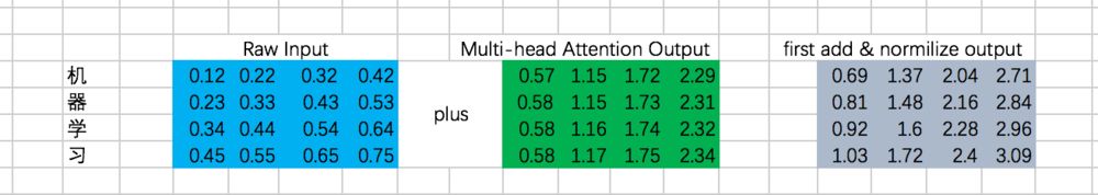
第一次Add & Normalize

接下來是一個FFN，我們仍然假設是固定的參數，那么output是：

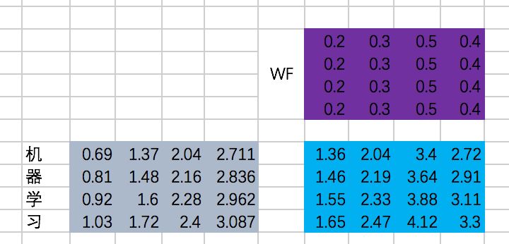
第二次Add & Normalize

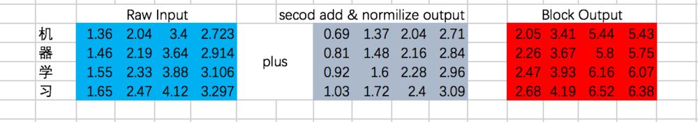
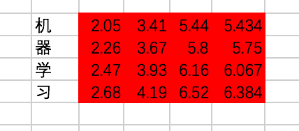
我們終于在經過一個Encoder的Block后得到了每個輸入對應的輸出，分別為：

讓我們把這段代碼補充上去吧：

with tf.variable_scope("encoder_block"): encoder_Q = tf.matmul(tf.reshape(encoder_embedding_input,(-1,tf.shape(encoder_embedding_input)[2])),w_Q) encoder_K = tf.matmul(tf.reshape(encoder_embedding_input,(-1,tf.shape(encoder_embedding_input)[2])),w_K) encoder_V = tf.matmul(tf.reshape(encoder_embedding_input,(-1,tf.shape(encoder_embedding_input)[2])),w_V) encoder_Q = tf.reshape(encoder_Q,(tf.shape(encoder_embedding_input)[0],tf.shape(encoder_embedding_input)[1],-1)) encoder_K = tf.reshape(encoder_K,(tf.shape(encoder_embedding_input)[0],tf.shape(encoder_embedding_input)[1],-1)) encoder_V = tf.reshape(encoder_V,(tf.shape(encoder_embedding_input)[0],tf.shape(encoder_embedding_input)[1],-1)) encoder_Q_split = tf.split(encoder_Q,2,axis=2) encoder_K_split = tf.split(encoder_K,2,axis=2) encoder_V_split = tf.split(encoder_V,2,axis=2) encoder_Q_concat = tf.concat(encoder_Q_split,axis=0) encoder_K_concat = tf.concat(encoder_K_split,axis=0) encoder_V_concat = tf.concat(encoder_V_split,axis=0) attention_map = tf.matmul(encoder_Q_concat,tf.transpose(encoder_K_concat,[0,2,1])) attention_map = attention_map / 8 attention_map = tf.nn.softmax(attention_map) weightedSumV = tf.matmul(attention_map,encoder_V_concat) outputs_z = tf.concat(tf.split(weightedSumV,2,axis=0),axis=2) sa_outputs = tf.matmul(tf.reshape(outputs_z,(-1,tf.shape(outputs_z)[2])),w_Z) sa_outputs = tf.reshape(sa_outputs,(tf.shape(encoder_embedding_input)[0],tf.shape(encoder_embedding_input)[1],-1)) sa_outputs = sa_outputs + encoder_embedding_input # todo :add BN W_f = tf.constant([[0.2,0.3,0.5,0.4], [0.2,0.3,0.5,0.4], [0.2,0.3,0.5,0.4], [0.2,0.3,0.5,0.4]]) ffn_outputs = tf.matmul(tf.reshape(sa_outputs,(-1,tf.shape(sa_outputs)[2])),W_f) ffn_outputs = tf.reshape(ffn_outputs,(tf.shape(sa_outputs)[0],tf.shape(sa_outputs)[1],-1)) encoder_outputs = ffn_outputs + sa_outputs # todo :add BNimport numpy as npwith tf.Session() as sess:# print(sess.run(encoder_Q))# print(sess.run(encoder_Q_split)) #print(sess.run(weightedSumV)) #print(sess.run(outputs_z)) #print(sess.run(sa_outputs)) #print(sess.run(ffn_outputs)) print(sess.run(encoder_outputs))

輸出為：

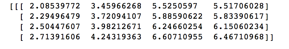
與excel計算結果基本一致。

當然，encoder的各層是可以堆疊的，但我們這里只以單層的為例，重點是理解整個過程。

3、Decoder Block

一個Decoder的Block過程如下：

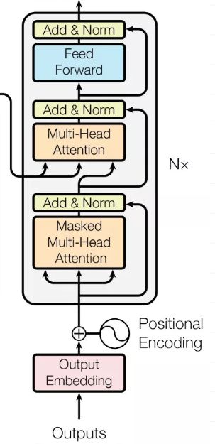
相比Encoder，這里的過程分為6步，分別是 masked multi-head self attention、Add & Normalize、encoder-decoder attention、Add & Normalize、Feed Forward Network、Add & Normalize。

咱們還是重點來講masked multi-head self attention和encoder-decoder attention。

3.1 Decoder輸入

這里，在excel中，咱們還是以第一條輸入為例，來展示整個過程：

[機、器、學、習] -> [ machine、learning]

因此，Decoder階段的輸入是：

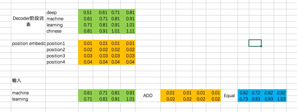
對應的代碼如下：

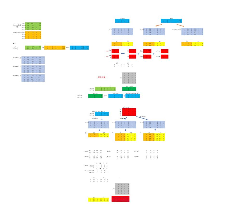
english_embedding = tf.constant([[0.51,0.61,0.71,0.81], [0.61,0.71,0.81,0.91], [0.71,0.81,0.91,1.01], [0.81,0.91,1.01,1.11]],dtype=tf.float32)position_encoding = tf.constant([[0.01,0.01,0.01,0.01], [0.02,0.02,0.02,0.02], [0.03,0.03,0.03,0.03], [0.04,0.04,0.04,0.04]],dtype=tf.float32)decoder_input = tf.constant([[1,2],[2,1]],dtype=tf.int32)with tf.variable_scope("decoder_input"): decoder_embedding_input = tf.nn.embedding_lookup(english_embedding,decoder_input) decoder_embedding_input = decoder_embedding_input + position_encoding[0:tf.shape(decoder_embedding_input)[1]]

3.2 masked multi-head self attention

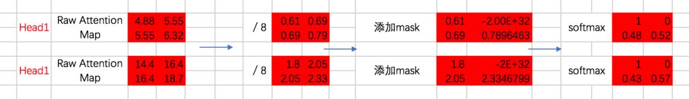
這個過程和multi-head self attention基本一致，只不過對于decoder來說，得到每個階段的輸出時，我們是看不到后面的信息的。舉個例子，我們的第一條輸入是：[機、器、學、習] -> [ machine、learning] ，decoder階段兩次的輸入分別是machine和learning，在輸入machine時，我們是看不到learning的信息的，因此在計算attention的權重的時候，machine和learning的權重是沒有的。我們還是先通過excel來演示一下，再通過代碼來理解：

計算Attention的權重矩陣是：

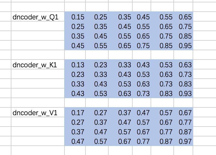
仍然以兩個Head為例，計算Q、K、V：

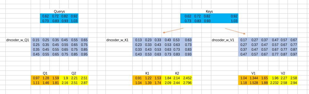
分別計算兩個Head的attention map

咱們先來實現這部分的代碼，masked attention map的計算過程：

先定義下權重矩陣，同encoder一樣，定義成常數：

w_Q_decoder_sa = tf.constant([[0.15,0.25,0.35,0.45,0.55,0.65], [0.25,0.35,0.45,0.55,0.65,0.75], [0.35,0.45,0.55,0.65,0.75,0.85], [0.45,0.55,0.65,0.75,0.85,0.95]],dtype=tf.float32)w_K_decoder_sa = tf.constant([[0.13,0.23,0.33,0.43,0.53,0.63], [0.23,0.33,0.43,0.53,0.63,0.73], [0.33,0.43,0.53,0.63,0.73,0.83], [0.43,0.53,0.63,0.73,0.83,0.93]],dtype=tf.float32)w_V_decoder_sa = tf.constant([[0.17,0.27,0.37,0.47,0.57,0.67], [0.27,0.37,0.47,0.57,0.67,0.77], [0.37,0.47,0.57,0.67,0.77,0.87], [0.47,0.57,0.67,0.77,0.87,0.97]],dtype=tf.float32)

隨后，計算添加mask之前的attention map：

with tf.variable_scope("decoder_sa_block"): decoder_Q = tf.matmul(tf.reshape(decoder_embedding_input,(-1,tf.shape(decoder_embedding_input)[2])),w_Q_decoder_sa) decoder_K = tf.matmul(tf.reshape(decoder_embedding_input,(-1,tf.shape(decoder_embedding_input)[2])),w_K_decoder_sa) decoder_V = tf.matmul(tf.reshape(decoder_embedding_input,(-1,tf.shape(decoder_embedding_input)[2])),w_V_decoder_sa) decoder_Q = tf.reshape(decoder_Q,(tf.shape(decoder_embedding_input)[0],tf.shape(decoder_embedding_input)[1],-1)) decoder_K = tf.reshape(decoder_K,(tf.shape(decoder_embedding_input)[0],tf.shape(decoder_embedding_input)[1],-1)) decoder_V = tf.reshape(decoder_V,(tf.shape(decoder_embedding_input)[0],tf.shape(decoder_embedding_input)[1],-1)) decoder_Q_split = tf.split(decoder_Q,2,axis=2) decoder_K_split = tf.split(decoder_K,2,axis=2) decoder_V_split = tf.split(decoder_V,2,axis=2) decoder_Q_concat = tf.concat(decoder_Q_split,axis=0) decoder_K_concat = tf.concat(decoder_K_split,axis=0) decoder_V_concat = tf.concat(decoder_V_split,axis=0) decoder_sa_attention_map_raw = tf.matmul(decoder_Q_concat,tf.transpose(decoder_K_concat,[0,2,1])) decoder_sa_attention_map = decoder_sa_attention_map_raw / 8

隨后，對attention map添加mask：

diag_vals = tf.ones_like(decoder_sa_attention_map[0,:,:])tril = tf.contrib.linalg.LinearOperatorTriL(diag_vals).to_dense()masks = tf.tile(tf.expand_dims(tril,0),[tf.shape(decoder_sa_attention_map)[0],1,1])paddings = tf.ones_like(masks) * (-2 ** 32 + 1)decoder_sa_attention_map = tf.where(tf.equal(masks,0),paddings,decoder_sa_attention_map)decoder_sa_attention_map = tf.nn.softmax(decoder_sa_attention_map)

這里我們首先構造一個全1的矩陣diag_vals，這個矩陣的大小同attention map。隨后通過tf.contrib.linalg.LinearOperatorTriL方法把上三角部分變為0，該函數的示意如下：

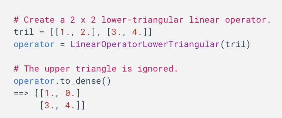
基于這個函數生成的矩陣tril，我們便可以構造對應的mask了。不過需要注意的是，對于我們要加mask的地方，不能賦值為0，而是需要賦值一個很小的數，這里為-2^32 + 1。因為我們后面要做softmax，e^0=1，是一個很大的數啦。

運行上面的代碼：

import numpy as npwith tf.Session() as sess: print(sess.run(decoder_sa_attention_map))

觀察第一條數據對應的結果如下：

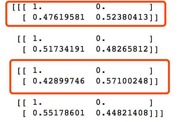
與我們excel計算結果相吻合。

后面的過程我們就不詳細介紹了，我們直接給出經過masked multi-head self attention的對應結果：

對應的代碼如下：

weightedSumV = tf.matmul(decoder_sa_attention_map,decoder_V_concat) decoder_outputs_z = tf.concat(tf.split(weightedSumV,2,axis=0),axis=2) decoder_sa_outputs = tf.matmul(tf.reshape(decoder_outputs_z,(-1,tf.shape(decoder_outputs_z)[2])),w_Z_decoder_sa) decoder_sa_outputs = tf.reshape(decoder_sa_outputs,(tf.shape(decoder_embedding_input)[0],tf.shape(decoder_embedding_input)[1],-1))with tf.Session() as sess: print(sess.run(decoder_sa_outputs))

輸出為：

與excel保持一致！

3.3 encoder-decoder attention

在encoder-decoder attention之間，還有一個Add & Normalize的過程，同樣，我們忽略 Normalize，只做Add操作：

接下來，就是encoder-decoder了，這里跟multi-head attention相同，但是需要注意的一點是，我們這里想要做的是，計算decoder的每個階段的輸入和encoder階段所有輸出的attention，所以Q的計算通過decoder對應的embedding計算，而K和V通過encoder階段輸出的embedding來計算：

接下來，計算Attention Map，注意，這里attention map的大小為2 * 4的，每一行代表一個decoder的輸入，與所有encoder輸出之間的attention score。同時，我們不需要添加mask，因為decoder的輸入是可以看到所有encoder的輸出信息的。得到的attention map結果如下：

哈哈，這里數是我瞎寫的，結果不太好，不過不影響對整個過程的理解。

接下來，我們得到整個encoder-decoder階段的輸出為：

接下來，還有Add & Normalize、Feed Forward Network、Add & Normalize過程，咱們這里就省略了。直接上代碼吧：

w_Q_decoder_sa2 = tf.constant([[0.2,0.3,0.4,0.5,0.6,0.7], [0.3,0.4,0.5,0.6,0.7,0.8], [0.4,0.5,0.6,0.7,0.8,0.9], [0.5,0.6,0.7,0.8,0.9,1]],dtype=tf.float32)w_K_decoder_sa2 = tf.constant([[0.18,0.28,0.38,0.48,0.58,0.68], [0.28,0.38,0.48,0.58,0.68,0.78], [0.38,0.48,0.58,0.68,0.78,0.88], [0.48,0.58,0.68,0.78,0.88,0.98]],dtype=tf.float32)w_V_decoder_sa2 = tf.constant([[0.22,0.32,0.42,0.52,0.62,0.72], [0.32,0.42,0.52,0.62,0.72,0.82], [0.42,0.52,0.62,0.72,0.82,0.92], [0.52,0.62,0.72,0.82,0.92,1.02]],dtype=tf.float32)w_Z_decoder_sa2 = tf.constant([[0.1,0.2,0.3,0.4], [0.1,0.2,0.3,0.4], [0.1,0.2,0.3,0.4], [0.1,0.2,0.3,0.4], [0.1,0.2,0.3,0.4], [0.1,0.2,0.3,0.4]],dtype=tf.float32)with tf.variable_scope("decoder_encoder_attention_block"): decoder_sa_outputs = decoder_sa_outputs + decoder_embedding_input encoder_decoder_Q = tf.matmul(tf.reshape(decoder_sa_outputs,(-1,tf.shape(decoder_sa_outputs)[2])),w_Q_decoder_sa2) encoder_decoder_K = tf.matmul(tf.reshape(encoder_outputs,(-1,tf.shape(encoder_outputs)[2])),w_K_decoder_sa2) encoder_decoder_V = tf.matmul(tf.reshape(encoder_outputs,(-1,tf.shape(encoder_outputs)[2])),w_V_decoder_sa2) encoder_decoder_Q = tf.reshape(encoder_decoder_Q,(tf.shape(decoder_embedding_input)[0],tf.shape(decoder_embedding_input)[1],-1)) encoder_decoder_K = tf.reshape(encoder_decoder_K,(tf.shape(encoder_outputs)[0],tf.shape(encoder_outputs)[1],-1)) encoder_decoder_V = tf.reshape(encoder_decoder_V,(tf.shape(encoder_outputs)[0],tf.shape(encoder_outputs)[1],-1)) encoder_decoder_Q_split = tf.split(encoder_decoder_Q,2,axis=2) encoder_decoder_K_split = tf.split(encoder_decoder_K,2,axis=2) encoder_decoder_V_split = tf.split(encoder_decoder_V,2,axis=2) encoder_decoder_Q_concat = tf.concat(encoder_decoder_Q_split,axis=0) encoder_decoder_K_concat = tf.concat(encoder_decoder_K_split,axis=0) encoder_decoder_V_concat = tf.concat(encoder_decoder_V_split,axis=0) encoder_decoder_attention_map_raw = tf.matmul(encoder_decoder_Q_concat,tf.transpose(encoder_decoder_K_concat,[0,2,1])) encoder_decoder_attention_map = encoder_decoder_attention_map_raw / 8 encoder_decoder_attention_map = tf.nn.softmax(encoder_decoder_attention_map) weightedSumV = tf.matmul(encoder_decoder_attention_map,encoder_decoder_V_concat) encoder_decoder_outputs_z = tf.concat(tf.split(weightedSumV,2,axis=0),axis=2) encoder_decoder_outputs = tf.matmul(tf.reshape(encoder_decoder_outputs_z,(-1,tf.shape(encoder_decoder_outputs_z)[2])),w_Z_decoder_sa2) encoder_decoder_attention_outputs = tf.reshape(encoder_decoder_outputs,(tf.shape(decoder_embedding_input)[0],tf.shape(decoder_embedding_input)[1],-1)) encoder_decoder_attention_outputs = encoder_decoder_attention_outputs + decoder_sa_outputs # todo :add BN W_f = tf.constant([[0.2,0.3,0.5,0.4], [0.2,0.3,0.5,0.4], [0.2,0.3,0.5,0.4], [0.2,0.3,0.5,0.4]]) decoder_ffn_outputs = tf.matmul(tf.reshape(encoder_decoder_attention_outputs,(-1,tf.shape(encoder_decoder_attention_outputs)[2])),W_f) decoder_ffn_outputs = tf.reshape(decoder_ffn_outputs,(tf.shape(encoder_decoder_attention_outputs)[0],tf.shape(encoder_decoder_attention_outputs)[1],-1)) decoder_outputs = decoder_ffn_outputs + encoder_decoder_attention_outputs # todo :add BNwith tf.Session() as sess: print(sess.run(decoder_outputs))

4、全連接層及最終輸出

最后的全連接層很簡單了，對于decoder階段的輸出，通過全連接層和softmax之后，最終得到選擇每個單詞的概率，并計算交叉熵損失：

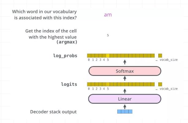
這里，我們直接給出代碼：

W_final = tf.constant([[0.2,0.3,0.5,0.4], [0.2,0.3,0.5,0.4], [0.2,0.3,0.5,0.4], [0.2,0.3,0.5,0.4]])logits = tf.matmul(tf.reshape(decoder_outputs,(-1,tf.shape(decoder_outputs)[2])),W_final)logits = tf.reshape(logits,(tf.shape(decoder_outputs)[0],tf.shape(decoder_outputs)[1],-1)) logits = tf.nn.softmax(logits)y = tf.one_hot(decoder_input,depth=4)loss = tf.nn.softmax_cross_entropy_with_logits(logits=logits,labels=y)train_op = tf.train.AdamOptimizer(learning_rate=0.0001).minimize(loss)

整個文章下來，咱們不僅通過excel實現了一遍transorform的正向傳播過程，還通過tf代碼實現了一遍。放兩張excel的抽象圖，就知道是多么浩大的工程了：

好了，文章最后，咱們再來回顧一下整個Transformer的結構：