? ? ? ? 簡單搭建自己的神經網絡

1. 模型闡述

假設我們有下面的一組數據

?

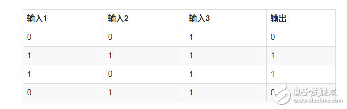
對于上面的表格，我們可以找出其中的一個規律是：

輸入的第一列和輸出相同

那對于輸入有3列，每列有0和1兩個值，那可能的排列有（2^3=8）種，但是此處只有4種，那么在有限的數據情況下，我們應該怎么預測其他結果呢？

看代碼：

%matplotlib inline

%config InlineBackend.figure_format = ‘retina’

from numpy import exp， array， random， dot

class NeuralNetwork（）：

def __init__（self）：

# Seed the random number generator， so it generates the same numbers

# every time the program runs.

random.seed（1）

# We model a single neuron， with 3 input connections and 1 output connection.

# We assign random weights to a 3 x 1 matrix， with values in the range -1 to 1

# and mean 0.

self.synaptic_weights = 2 * random.random（（3， 1）） - 1

self.sigmoid_derivative = self.__sigmoid_derivative

# The Sigmoid function， which describes an S shaped curve.

# We pass the weighted sum of the inputs through this function to

# normalise them between 0 and 1.

def __sigmoid（self， x）：

return 1 / （1 + exp（-x））

# The derivative of the Sigmoid function.

# This is the gradient of the Sigmoid curve.

# It indicates how confident we are about the existing weight.

def __sigmoid_derivative（self， x）：

return x * （1 - x）

# We train the neural network through a process of trial and error.

# Adjusting the synaptic weights each time.

def train（self， training_set_inputs， training_set_outputs， number_of_training_iterations）：

for iteration in range（number_of_training_iterations）：

# Pass the training set through our neural network （a single neuron）。

output = self.think（training_set_inputs）

# Calculate the error （The difference between the desired output

# and the predicted output）。

error = training_set_outputs - output

# Multiply the error by the input and again by the gradient of the Sigmoid curve.

# This means less confident weights are adjusted more.

# This means inputs， which are zero， do not cause changes to the weights.

adjustment = dot（training_set_inputs.T， error * self.__sigmoid_derivative（output））

# Adjust the weights.

self.synaptic_weights += adjustment

# The neural network thinks.

def think（self， inputs）：

# Pass inputs through our neural network （our single neuron）。

return self.__sigmoid（dot（inputs， self.synaptic_weights））

#Intialise a single neuron neural network.

neural_network = NeuralNetwork（）

print（“Random starting synaptic weights： ”）

print（neural_network.synaptic_weights）

# The training set. We have 4 examples， each consisting of 3 input values# and 1 output value.

training_set_inputs = array（［［0， 0， 1］， ［1， 1， 1］， ［1， 0， 1］， ［0， 1， 1］］）

training_set_outputs = array（［［0， 1， 1， 0］］）.T

# Train the neural network using a training set.# Do it 10，000 times and make small adjustments each time.

neural_network.train（training_set_inputs， training_set_outputs， 10000）

print（“New synaptic weights after training： ”）

print（neural_network.synaptic_weights）

# Test the neural network with a new situation.

print（“Considering new situation ［1， 0， 0］ -》 ？： ”）

print（neural_network.think（array（［1， 0， 0］）））

Random starting synaptic weights： ［［-0.16595599］

［ 0.44064899］

［-0.99977125］］

New synaptic weights after training： ［［ 9.67299303］

［-0.2078435 ］

［-4.62963669］］

Considering new situation ［1， 0， 0］ -》 ？： ［ 0.99993704］

以上代碼來自：https://github.com/llSourcell/Make_a_neural_network

現在我們來分析下具體的過程：

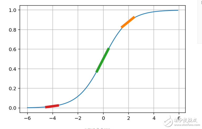
第一個我們需要注意的是sigmoid function，其圖如下：

import matplotlib.pyplot as pltimport numpy as np

def sigmoid（x）：

a = ［］

for item in x：

a.append（1/（1+np.exp（-item）））

return a

x = np.arange（-6.， 6.， 0.2）

sig = sigmoid（x）

plt.plot（x，sig）

plt.grid（）

plt.show（）

?

我們可以看到sigmoid函數將輸入轉換到了0-1之間的值，而sigmoid函數的導數是：

def __sigmoid_derivative（self， y）：

return y * （1 - y）

其具體的含義看圖：

def sigmoid_derivative（x）：

y = 1/（1+np.exp（-x））

return y * （1-y）

def derivative（point）：

dx = np.arange（-0.5，0.5，0.1）

slope = sigmoid_derivative（point）

return ［point+dx，slope * dx + 1/（1+np.exp（-point））］

x = np.arange（-6.， 6.， 0.1）

sig = sigmoid（x）

point1 = 2

slope1 = sigmoid_derivative（point1）

plt.plot（x，sig）

x1，y1 = derivative（point1）

plt.plot（x1，y1，linewidth=5）

x2，y2 = derivative（0）

plt.plot（x2，y2，linewidth=5）

x3，y3 = derivative（-4）

plt.plot（x3，y3，linewidth=5）

plt.grid（）

plt.show（）

?

現在我們來根據圖解釋下實際的含義：

1. 首先輸出是0到1之間的值，我們可以將其認為是一個可信度，0不可信，1完全可信

2. 當輸入是0的時候，輸出是0.5，什么意思呢？意思是輸出模棱兩可

基于以上兩點，我們來看下上面函數的中的一個計算過程：

adjustment = dot（training_set_inputs.T， error * self.__sigmoid_derivative（output））

這個調整值的含義我們就知道了，當輸出接近0和1時候，我們已經預測的挺準了，此時調整就基本接近于0了

而當輸出為0.5左右的時候，說明預測完全是瞎猜，我們就需要快速調整，因此此時的導數也是最大的，即上圖的綠色曲線，其斜度也是最大的

基于上面的一個討論，我們還可以有下面的一個結論：

1. 當輸入是1，輸出是0，我們需要不斷減小 weight 的值，這樣子輸出才會是很小，sigmoid輸出才會是0

2. 當輸入是1，輸出是1，我們需要不斷增大 weight 的值，這樣子輸出才會是很大，sigmoid輸出才會是1

這時候我們再來看下最初的數據，

?

我們可以斷定輸入1的weight值會變大，而輸入2，3的weight值會變小。

根據之前訓練出來的結果也支持了我們的推斷：

2. 擴展

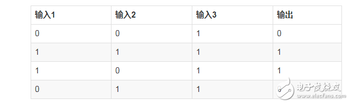
我們來將上面的問題稍微復雜下，假設我們的輸入如下：

?

此處我們只是改變一個值，此時我們再次訓練呢？

我們觀察上面的數據，好像很難再像最初一樣直接觀察出 輸出1 == 輸出 的這種簡單的關系了，我們要稍微深入的觀察下了

· 首先輸入3都是1，看起來對輸出沒什么影響

· 接著觀察輸入1和輸入2，似乎只要兩者不同，輸出就是1

基于上面的觀察，我們似乎找不到像輸出1 == 輸出這種 one-to-one 的關系了，我們有什么辦法呢？

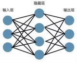
這個時候，就需要引入 hidden layer，如下表格：

?

此時我們得到中的中間輸入和最后輸出就還是原來的一個 輸出1 == 輸出 關系了。

上面介紹的這種方法就是深度學習的最簡單的形式

深度學習就是通過增加層次，不斷去放大輸入和輸出之間的關系，到最后，我們可以從復雜的初看起來毫不相干的數據中，找到一個能一眼就看出來的關系

此處我們還是用之前的網絡來訓練

?

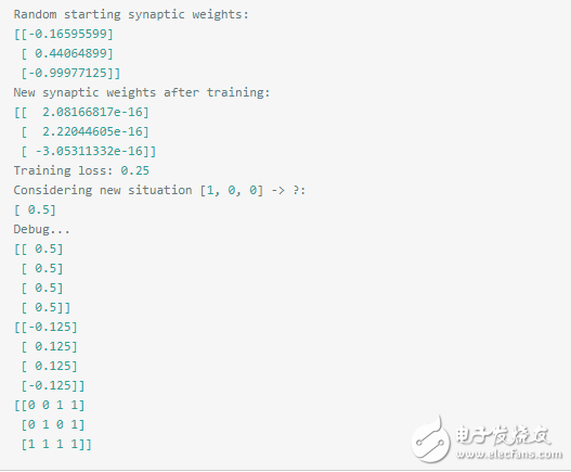
此處我們訓練可以發現，此處的誤差基本就是0.25，然后預測基本不可信。0.5什么鬼！

由數據可以看到此處的weight都已經非常非常小了，然后斜率是0.5，

由上面打印出來的數據，已經達到平衡，adjustment都是0了，不會再次調整了。

由此可以看出，簡單的一層網絡已經不能再精準的預測了，只能增加復雜度了。

下面我們來加一層再來看下：

class TwoLayerNeuralNetwork（object）：

def __init__（self， input_nodes， hidden_nodes， output_nodes， learning_rate）：

# Set number of nodes in input， hidden and output layers.

self.input_nodes = input_nodes

self.hidden_nodes = hidden_nodes

self.output_nodes = output_nodes

np.random.seed（1）

# Initialize weights

self.weights_0_1 = np.random.normal（0.0， self.hidden_nodes**-0.5，

（self.input_nodes， self.hidden_nodes）） # n * 2

self.weights_1_2 = np.random.normal（0.0， self.output_nodes**-0.5，

（self.hidden_nodes， self.output_nodes）） # 2 * 1

self.lr = learning_rate

#### Set this to your implemented sigmoid function ####

# Activation function is the sigmoid function

self.activation_function = self.__sigmoid

def __sigmoid（self， x）：

return 1 / （1 + np.exp（-x））

def __sigmoid_derivative（self， x）：

return x * （1 - x）

def train（self， inputs_list， targets_list）：

# Convert inputs list to 2d array

inputs = np.array（inputs_list，ndmin=2） # 1 * n

layer_0 = inputs

targets = np.array（targets_list，ndmin=2） # 1 * 1

#### Implement the forward pass here ####

### Forward pass ###

layer_1 = self.activation_function（layer_0.dot（self.weights_0_1）） # 1 * 2

layer_2 = self.activation_function（layer_1.dot（self.weights_1_2）） # 1 * 1

#### Implement the backward pass here ####

### Backward pass ###

# TODO： Output error

layer_2_error = targets - layer_2

layer_2_delta = layer_2_error * self.__sigmoid_derivative（layer_2）# y = x so f‘（h） = 1

layer_1_error = layer_2_delta.dot（self.weights_1_2.T）

layer_1_delta = layer_1_error * self.__sigmoid_derivative（layer_1）

# TODO： Update the weights

self.weights_1_2 += self.lr * layer_1.T.dot（layer_2_delta） # update hidden-to-output weights with gradient descent step

self.weights_0_1 += self.lr * layer_0.T.dot（layer_1_delta） # update input-to-hidden weights with gradient descent step

def run（self， inputs_list）：

# Run a forward pass through the network

inputs = np.array（inputs_list，ndmin=2）

#### Implement the forward pass here ####

layer_1 = self.activation_function（inputs.dot（self.weights_0_1）） # 1 * 2

layer_2 = self.activation_function（layer_1.dot（self.weights_1_2）） # 1 * 1

return layer_2def MSE（y， Y）：

return np.mean（（y-Y）**2）

# import sys

training_set_inputs = array（［［0， 0， 1］， ［0， 1， 1］， ［1， 0， 1］， ［1， 1， 1］］）

training_set_outputs = array（［［0， 1， 1， 0］］）.T

### Set the hyperparameters here ###

epochs = 20000

learning_rate = 0.1

hidden_nodes = 4

output_nodes = 1

N_i = 3

network = TwoLayerNeuralNetwork（N_i， hidden_nodes， output_nodes， learning_rate）

losses = {’train‘：［］}for e in range（epochs）：

# Go through a random batch of 128 records from the training data set

for record， target in zip（training_set_inputs，

training_set_outputs）：# print（target）

network.train（record， target）

train_loss = MSE（network.run（training_set_inputs）， training_set_outputs）

sys.stdout.write（“ Progress： ” + str（100 * e/float（epochs））［：4］

+ “% 。。。 Training loss： ” + str（train_loss）［：7］）

losses［’train‘］.append（train_loss）

print（“ ”）

print（“After train，layer_0_1： ”）

print（network.weights_0_1）

print（“After train，layer_1_2： ”）

print（network.weights_1_2）# Test the neural network with a new situation.

print（“Considering new situation ［1， 0， 0］ -》 ？： ”）

print（network.run（array（［1， 0， 0］）））

Progress： 99.9% 。。。 Training loss： 0.00078

After train，layer_0_1：

［［ 4.4375838 -3.87815184 1.74047905 -5.12726884］

［ 4.43114847 -3.87644617 1.71905492 -5.10688387］

［-6.80858063 0.76685389 1.89614363 1.61202043］］

After train，layer_1_2：

［［-9.21973137］

［-3.84985864］

［ 4.75257888］

［-6.36994226］］

Considering new situation ［1， 0， 0］ -》 ？：

［［ 0.00557239］］

layer_1=network.activation_function（training_set_inputs.dot（network.weights_0_1））

print（layer_1）

layer_2 = network.activation_function（layer_1.dot（network.weights_1_2））

print（layer_2）

［［ 2.20482250e-01 9.33639853e-01 6.30402293e-01 6.24775766e-02］

［ 1.77659862e-02 9.99702482e-01 8.64290928e-01 9.26611880e-01］

［ 6.94975743e-01 8.90040645e-02 8.51261229e-01 2.06917379e-04］

［ 1.27171786e-01 9.58904341e-01 9.55296949e-01 3.77322214e-02］］

［［ 0.02374213］

［ 0.97285992］

［ 0.97468116］

［ 0.02714965］］

最后總結：我們發現在擴展中，我們只是簡單的改變了兩個輸入值，此時再次用一層神經網絡已經難以預測出正確的數據了，此時我們只能通過將神經網絡變深，這個過程其實就是再去深度挖掘數據之間關系的過程，此時我們的2層神經網絡相比較1層就好多了。